House Prices Prediction
Keywords: linear regression, tableau, pandas, numpy, sklearn
This project is my solution to Kaggle House Prices - Advanced Regression Techniques competition. The test and train data can be found in the Kaggle page. The source code of my approach can be found in House Prices Prediction.
In the competition, properties and prices of >1000 houses are given as training data. Competition asks us to predict prices of houses in the test data. Data has 81 columns, one of which is the ID column and one is the price columns. Hence, we have to predict the price of an house using 79 columns. 46 of the 79 columns are categorical, while the 33 remaining are continuous.
An example categorical column is MSZoning which identifies the general zoning classification of the house. It takes a value from [Agriculture, Commercial, Floating Village Residential, Industrial, Residential High Density, Residential Low Density, Residential Low Density Park, Residential Medium Density].
I solve this problem using linear regression.
Cleaning the Data
Since the number of columns are large and the data is detailed, I started with deciding what the unnecessary columns are. I sketched the graphs of sale prices for every categorical column using Tableau. I observed that some of the columns are unnecessary. These columns are:
- Street: Type of road access to property (Gravel or Paved)
- Utilities: Type of utilities available (All utilities, no sewer, no sewer and water, or electricity only)
- Condition2: Proximity to various conditions (Adjacent to arterial street, Adjacent to feeder street, etc.)
- Heating: Type of heating (Floor Furnace, Gas forced warm air furnace, etc.)
- PoolQC: Pool quality (Excellent, Good, etc.)
- MoSold: Month Sold (MM)
- YrSold: Year Sold (YYYY)
- GarageYrBlt: Year garage was built
- Alley: Type of alley access to property (Gravel, Paved, No alley access)
- LotConfig: Lot configuration (Inside lot, Corner lot, etc.)
- LandSlope: Slope of property (Gentle, Moderate, Severe)
- GarageFinish: Interior finish of the garage (Finished, Rough Finished, etc.)
Removing each of these columns individually improved the performance of the linear regressor. I will give a brief explanation of why I chose these columns in the first place.
MoSold and YrSold Columns
First, MoSold and YrSold represent month and year the houses were sold. In the data, all of the houses are sold between years 2007-2010. Since the US inflation rate was close to 0% in those years, these columns seemed irrelevant.
Street Column
In the Street column, there are only 6 houses that have an access to property with a gravel road. The rest of the houses (1454 houses in total) use paved roads. There are significantly small amount of houses that has an access with a gravel road. Hence, they are outliers. Instead of losing those houses completely, I chose to remove the street column as that column is the reason of them being outliers.
Utilities Column
In the Utilities column, there is only one house that has only electricity and gas. All the others have all utilities. So, this column also should not affect our decision significantly. Therefore, I dropped it.
Condition2 Column
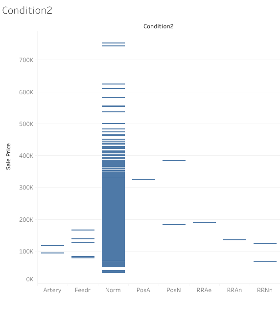
In the Condition2 column (see image below), almost all of the houses have normal condition. Since this is an another column that should not effect the overall behavior of the model, I dropped it.
Heating Column
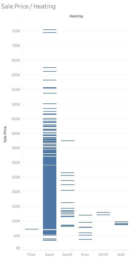
In the Heating column, the data is scattered with the majority belonging to GasA (see image below). The significantly small number of houses, about %5 of them, are using other heating choices. I was skeptical about dropping this column, but since deleting this column resulted in a better model, I dropped it in the end.
PoolQC Column
Since only 7 houses has a pool in the training data, having non-NA value this column makes houses outliers. Therefore, I removed the column.
GarageYrBlt Column
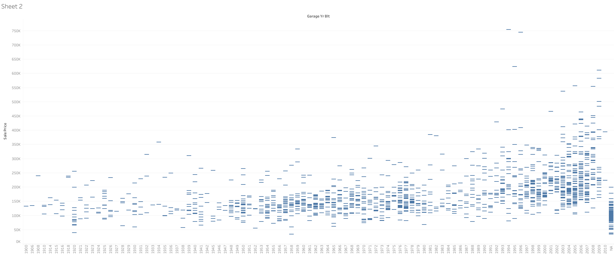
This column includes the year the garage of the house is built. Looking at the graph of GarageYrBlt vs price (see image below), there seems to be a slight linear relation that price increases as GarageYrBlt increases. However, removing this column resulted in better quality of the trained model. Therefore, I chose to remove it.
Alley Column
>90% has NA value in this column, therefore I dropped it.
LotConfig Column
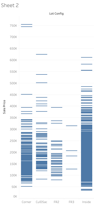
There is no clear linear relation between lot configuration and the price of the house (see image below). Therefore, I dropped the column.
LandSlope Column
When houses that have more than 500k sale price (which can be considered outliers because they constitude less than 2% of the dataset) are not considered, LandSlope column does not say a lot about the sale price of the house (see image below). Therefore, I dropped the column.

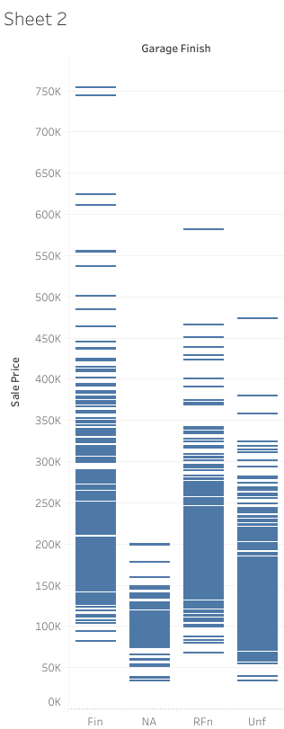
GarageFinish Column
When the houses that do not have a garage are considered, this column does not provide a distiguishing signal for the result. Therefore, I removed it. Even if there is a slight difference in means with different garage finishes (see image below), removing this column resulted in a better performing model.
Code
I use pandas.DataFrame to store data.
First, I define some helper functions in helpers.py file. remove_columns is the first function. It takes a pandas.DataFrame and a list of column names as argument, drops them from the pandas.DataFrame and returns a new pandas.DataFrame.
def remove_columns(data_frame, column_list):
    """
      This function takes a data_frame, removes columns
      given in column_list and returns the result as a
      new data frame
    """
    data_frame_with_remaining_columns = data_frame.drop(column_list, axis=1)
    return data_frame_with_remaining_columns
Next is the linear_regression function, which takes a pandas.DataFrame and a column name as an argument, and fits a linear model to columns in the pandas.DataFrame to predict the given column using sklearn.linear_model.LinearRegression. It returns the learned model, and the order of columns used in the regression. Column order is used at the test time to make sure that the model is used in a correct way. Columns of the test data are reordered with the returned column order.
from sklearn.linear_model import LinearRegression

def linear_regression(data_frame, output_column_name):
    """
      Given data_frame and output_column_name, fits a linear
      model to columns in the data_frame to predict the
      column with name output_column_name.

      Returns the learned model and the order of column names
      used in the regression.
    """
    X = data_frame.drop(output_column_name, axis=1)
    y = data_frame[output_column_name]
    reg = LinearRegression().fit(X, y)
    return reg, X.columns
In the main body of the code, I first import the required libraries.
import pandas as pd  # data processing, CSV file I/O (e.g. pd.read_csv).
from pandas.core.frame import DataFrame # Data format.
import numpy as np
from helpers import *
Then, I read the data, add a Bias column for linear regression, and drop unnecessary columns (listed above).
train_data_path = 'C:\\Users\\sevgi\\OneDrive\\Masaüstü\\Kaggle Housing Prices Competition\\train.csv'
train_data = pd.read_csv(train_data_path)
train_data['Bias'] = 1

copy_of_train_data = train_data.copy()
copy_of_train_data = remove_columns(copy_of_train_data, ["Id"])
unnecessary_columns = ['Street', 'Utilities', 'Condition2', 'Heating', 'PoolQC',
                       'MoSold', 'YrSold', 'GarageYrBlt', 'Alley', 'LotConfig',
                       'LandSlope', 'GarageFinish']
copy_of_train_data = remove_columns(copy_of_train_data, unnecessary_columns)
Some of the remaining columns of the data are categorical, while others are continuous. For the categorical columns, I create dummies that adds a distinct column for each value of each categorical column. When the categorical column is a particular value in a row, its corresponding column in dummies is set to 1, and all other dummies for that column are set to 0. You can read this article at Medium to learn more about dummies.
For the numerical columns (i.e., columns that are not categorical), I fill NA values with 0s in the way.
I list all categorical columns, and create dummies for each categorical column that is not unnecessary.
categorical_columns = ['MSSubClass', 'MSZoning', 'Street', 'LotShape',
                       'LandContour', 'Utilities', 'LotConfig', 'LandSlope',
                       'Neighborhood', 'Condition1', 'Condition2', 'BldgType',
                       'HouseStyle', 'OverallQual', 'OverallCond', 'RoofStyle',
                       'RoofMatl', 'Exterior1st', 'Exterior2nd', 'MasVnrType',
                       'ExterQual', 'ExterCond', 'Foundation', 'BsmtCond', 'BsmtExposure',
                       'BsmtFinType1', 'BsmtFinType2', 'BsmtQual', 'Heating',
                       'HeatingQC', 'CentralAir', 'Electrical', 'KitchenQual',
                       'Functional', 'FireplaceQu', 'GarageType', 'GarageFinish',
                       'GarageQual', 'GarageCond', 'PavedDrive', 'PoolQC',
                       'Fence', 'MiscFeature', 'SaleType', 'SaleCondition']
categorical_columns = list(set(categorical_columns) - set(unnecessary_columns))
numerical_columns = list(set(copy_of_train_data.columns) - set(categorical_columns))
copy_of_train_data[numerical_columns] = copy_of_train_data[numerical_columns].fillna(0)
copy_of_train_data = pd.get_dummies(copy_of_train_data, dummy_na=False, columns=categorical_columns)
dummy_na argument of pd.get_dummies includes NA values as a distinct category when set to true, and ignores NA values when set to false. I set it to false here in order to ignore NA values because it resulted in a better model.
Then, I apply linear regression to the data frame to predict SalePrice column.
model, column_order = linear_regression(copy_of_train_data, "SalePrice")I read the test data in the same way I read train data and add the Bias term. Then, I remove the unecesssary columns, remove the “SalePrice” column, fill NA values in numerical columns with 0, and get dummies for the categorical columns.
test_data_path = 'C:\\Users\\sevgi\\OneDrive\\Masaüstü\\Kaggle Housing Prices Competition\\test.csv'
test_data = pd.read_csv(test_data_path)
test_data['Bias'] = 1
copy_of_test_data = test_data.copy()
copy_of_test_data = remove_columns(copy_of_test_data, unnecessary_columns)
numerical_columns.remove("SalePrice")
copy_of_test_data[numerical_columns] = copy_of_test_data[numerical_columns].fillna(0)
copy_of_test_data = pd.get_dummies(copy_of_test_data, dummy_na = False, columns = categorical_columns)
If there are some categorical values in train data that do not appear in the test data, there will be no dummy for them in the test data. For those columns, I add them manually and set their values to 0, indicating that no row in test data has those particular values in the corresponding columns.
missing_columns_in_test_data = list(set(copy_of_train_data.columns) - set(copy_of_test_data.columns))
copy_of_test_data[missing_columns_in_test_data] = 0
Last, I predict the SalePrice’s of each row in the test data, and write result to result.csv file.
predicted_sale_prices = model.predict(copy_of_test_data[column_order])

result = pd.DataFrame()
result["Id"] = copy_of_test_data["Id"]
result["SalePrice"] = predicted_sale_prices

result_file = open("result.csv", "w")
result_file.write(result.to_csv(columns=["Id", "SalePrice"], line_terminator="\n", index=False))
result_file.close()
Performance
Kaggle judge system requires result.csv file and compares SalePrices to the secret SalePrices it has for the challenge. It reports the root mean squared logarithmic error between submitted answers and the real prices. My approach achieved RMSLE of 0.17439.